By Jaan Kalda (TalTech).
Let us start with a few observations. First, the frame rate is apparently so high that the effect of free fall acceleration is minimal and can be neglected when the number of frames involved is not large. Second, the water dynamics become extremely complicated very quickly, so that later frames are basically useless to us. Essentially, the only thing that can be reliably measured and used (based on a few frames before and a few frames after the impact) is the instantaneous change in speed of the cylinder during the impact.
This brings us to the question of what happens at the moment of impact. The cylinder hits the surface of the water, creates a huge pressure in the water below it at the moment of impact, and sets the water into motion almost instantaneously. Water flowing around moving submerged objects carries energy. In such cases, the energy of the water can be quantified by the added mass M_{\mathrm{added}} of the body. The question is, what happens during our impact? It is clear that during the very short period of the impact, the water begins to move in the same way as it would around a submerged moving body, so the energy of the water becomes almost instantaneously equal to M_{\mathrm{added}}v^2/2, where v is the velocity of the body after the impact. This means that water behaves like a rigid body with mass M_{\mathrm{added}}. A collision between two bodies can be elastic or plastic; in the former case, the two bodies would move away from each other after the collision at the same relative speed as before the collision. Here, however, the relative velocity after the collision is zero, just as in a perfectly plastic collision. Such a collision is described by the equation
M_{\mathrm{cyl}}u=(M_{\mathrm{cyl}}+M_{\mathrm{added}})v,
where u and v denote the speed of the cylinder immediately before and after the impact, respectively. If we were able to express M_{\mathrm{added}} in terms of the dimensions of the disc, we could use this equality to determine the density of the disc by measuring from the video the velocities before and after the impact.
The previous paragraph may seem a little unconvincing to readers who prefer rigour: we have drawn an analogy with a plastic collision without really talking about the momentum of the water, whereas it is the total momentum of the system that is conserved in a plastic collision. The reason is that the situation with momentum is a bit tricky. Consider a body moving from left to right in a tank of water at speed v. We can think of the body as a missing volume of water, i.e. a volume of density -\rho_w superimposed on the density of water +\rho_w. The centre of mass of the full tank remains at rest; the missing water volume V moves from left to right, so the centre of mass moves from right to left – opposite to the momentum of the moving body. The momentum of the water is therefore -\rho_vVv and does not depend on the added mass. Similarly, when the falling cylinder hits the surface of the water, the total momentum of the water is directed upwards; this momentum was created by the pressure force exerted by the bottom of the container. So we can see that (a) the direction of the total momentum of the water is “wrong”, opposite to what the impact with the disc would produce, and (b) it is caused by the walls, so it cannot be used to write down the effective conservation of momentum of the cylinder.
For those readers who were not convinced by how we arrived at the conservation of effective momentum, here is a more rigorous analysis. Consider the Euler equation for fluid dynamics,
\frac{\partial}{\partial t}\vec v+(\vec v\cdot\nabla)\vec v+\rho^{-1}\nabla p=0.During the impact, the pressure p and the time derivative \frac{\partial}{\partial t} take on very large values in a very short time. Let us integrate the Euler equation over the period of the impact, assuming that the velocity of the water was zero everywhere before the impact:
\rho\vec v+\nabla P=0, where P=\int p\mathrm dt.
Note that the second term of the Euler equation has disappeared because it remained much smaller than the other two terms during the impact. Let us now square the two sides of this equation and integrate over space:
Here we have integrated by parts and used the Gauss theorem. If we take the divergence of the previously obtained equality \rho\vec v+\nabla P=0 and remember that the \mathrm{div}\vec v=0, we obtain \nabla^2 P=0,. This simplifies the previous equation to \rho^2\int v^2\mathrm d^3\vec r=\oint P\nabla P\cdot\vec{\mathrm dA}; here we can replace \nabla P=-\rho\vec v, to get \rho\int v^2\mathrm d^3\vec r=-\oint P\vec v\cdot\vec{\mathrm dA}. Suppose we have integrated over a large volume, from the water surface downwards, over distances much greater than the dimension of the disc. At large distances, the velocity vanishes as a dipole field (this is shown below), i.e. as the distance cubed. Hence the surface integral vanishes over distant parts; at the free water surface, the pressure P under the integral is zero (because the pressure there is equal to the atmospheric pressure). At the surface of the disc, the normal component of the velocity of the water is equal to the velocity v of the disc; the left-hand side of this equation is the double kinetic energy of the water. So we get M_{\mathrm {added}}v^2=v\int P\mathrm dA, where the integral is taken over the contact surface between the disc and the water, or equivalently, M_{\mathrm{added}}v=\int P\mathrm dA=\int \left(\int p\mathrm dA\right)\mathrm dt=\int F\mathrm dt, where F=F(t) is the pressure force between the water and the disc. Because of Newton’s second law, the last integral gives us the change in momentum of the disc, i.e. we have proved that M_{\mathrm {added}}v is equal to the change in momentum of the disc.
So we have learned that what we have here is effectively a plastic collision between the disc and the added mass. Plastic collision means that energy has to be dissipated somewhere/somehow at the moment of impact. There is no viscous friction here (which could cause energy loss) because that would require shear flow, but as discussed above, our flow is potential. However, there is another mechanism by which excess energy can be released – sound waves in water. We’ll leave the discussion of the effect of sound waves for the end of this analysis.
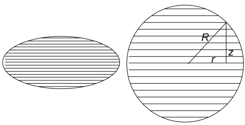
Next, we return to the task of expressing the added mass M_{\mathrm{added}} in terms of the dimensions of the cylinder. Normally the added mass is calculated for bodies moving in an infinite water tank. Here, however, the situation is a little more complicated: at the start, we have only a small part of the front of the cylinder immersed in the water. This means that the effect of the cylinder on the water is the same as that of an infinitely thin disc. When an infinitely thin disc moves in water, the streamlines in the plane of the disc are parallel to the axis of the cylinder (let this be the u-axis), due to up-and-down symmetry; this is illustrated in the figure below. In our case, only half of the space is filled with water, and the disc is just at the edge of the water volume, at x=0 . It appears that at x=0 the velocity of the water particles is also parallel to the x-axis, so the streamlines have the same shape as in the case of an infinite volume of water. The only difference from the infinite volume case is that the part x<0 is removed, i.e. half of the kinetic energy of the water is “cut away”. This means that the added mass is reduced by exactly two times. The reason why at x=0 the velocity of the water particles is parallel to the x-axis is that the surface of the water at x=0 is in direct contact with the surrounding air and therefore the pressure immediately below the surface is equal to the atmospheric pressure. Therefore, there can be no horizontal pressure gradients at x=0, so the water must start moving parallel to the x-axis.

In order to express the added mass of an infinitely thin disc, knowledge of hydrodynamics is required. The equations governing hydrodynamics in simpler cases are isomorphic to those governing electromagnetism, so we can use this analogy. Water is incompressible, so \oint \mathbf{v}\cdot\mathrm d\mathbf{A}=0. Water is initially motionless and the acceleration of water particles is caused by a pressure gradient which is a potential force field, hence the velocity field remains also to be a potential field, \oint \mathbf{v}\cdot\mathrm d\mathbf{l}=0.. These form exactly the same set of equations that we get from the Maxwell equations for electric and magnetic fields in a vacuum (when there are no currents and no charges). So, if we can match the boundary conditions, we can use the known solutions for electric or magnetic fields.
When a body is moving in water, it is convenient to use the co-moving frame in which the body is at rest. The incompressibility condition implies that the normal to the body surface component of the water velocity is zero. This is exactly the same condition that applies to the magnetic field at the surface of a superconductor (magnetic flux cannot cross the surface). To be clearer, if \mathbf{v}(\mathbf{r}) denotes the velocity field in water when the bulk of the water is at rest, and the disc is moving with velocity \mathbf{v}_0, then in the co-moving frame the velocity field is given by \mathbf{v}(\mathbf{r})-\mathbf v_0; which is matched to the magnetic field \mathbf{B}(\mathbf{r})-\mathbf B_0 around a superconducting disk in a homogeneous magnetic field \mathbf B_0, where \mathbf{B}(\mathbf{r}) is the field generated by the magnetised disk. Our new task is to express the magnetic energy of the field \mathbf{B}(\mathbf{r}) in terms of \mathbf B_0.
Instead of a disc, it is better to consider a superconducting ellipsoid (spheroid) and let the thickness of the spheroid be zero. The reason is that the ellipsoid is a shape that obeys a very special property: the magnetic field inside a homogeneously magnetised ellipsoid is also homogeneous. A superconducting body conserves magnetic flux through any closed loop inside itself; therefore, once placed inside a homogeneous magnetic field, the net magnetic field inside it must be zero. In the case of an ellipsoid, this means that the ellipsoid becomes homogeneously magnetised, with such a magnetization \mathbf J that the homogeneous field generated by the magnetised ellipsoid inside itself exactly compensates for the external homogeneous field.
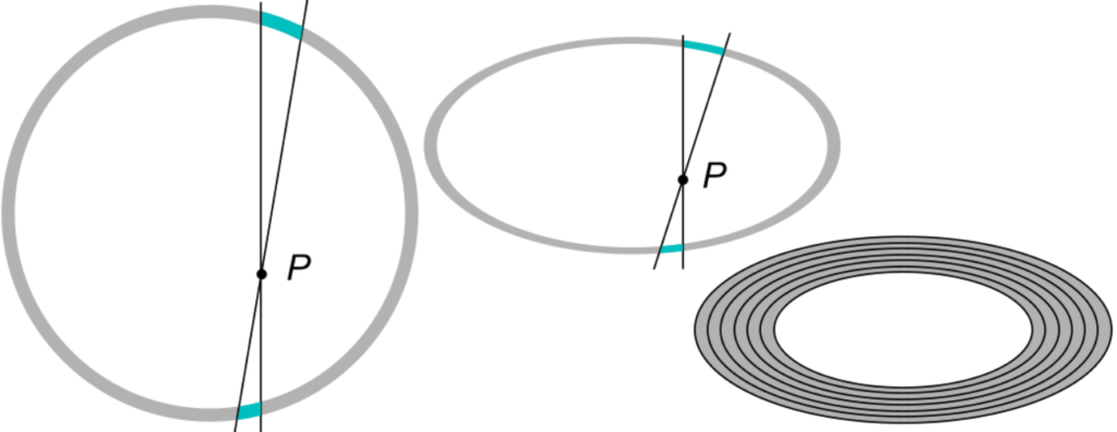
To show this property of ellipsoids, we start with a homogeneously charged spherical shell. It is well known, and follows directly from Gauss’s law and spherical symmetry, that the electric field inside such a shell is zero. The fact that it is zero can also be shown using another idea dating back to Isaac Newton. First we consider a homogeneously charged thin spherical shell as shown in the left figure below, select an arbitrary point P inside it, and cut two small opposing pieces (cyan in the figure) from the shell with two narrow cones as shown below. The total charges of these two pieces relate to each other as the square of the distance from point P, so the respective electric fields at P cancel each other out exactly. Since the whole shell can be divided into opposite pairs of charges, the total field at P is zero. It is easy to see that this cancellation remains valid if we perform an affine transformation on this spherical shell, transforming it into an ellipsoidal shell – a layer between two similar ellipsoids. Indeed, affine transformations preserve the ratio of the heights of the cones, as well as the ratio of the charges of the slices. The fields due to these charges cut from the shell by the cones (shown in blue) compensate exactly each other. The fields due to these charges cut by the cones (shown in blue) exactly cancel each other out. Finally, we note that the ellipsoidal shell need not be thin: a thick shell can be divided into a large number of thin shells, as shown in the figure on the right.
Let us now consider an ellipsoid with a homogeneous volume density of charges \rho_q; let its centre be O, and let us find the electric potential \varphi_(x,y,z) of a point P inside the ellipsoid; the potential of point O is taken to be zero. Next, we fictitiously mark a small ellipsoid of similar shape inside the large ellipsoid. Let the linear size of the small ellipsoid be k\gg 1 times smaller than that of the large ellipsoid. Consider the electric potential of point P’ with coordinates latex[/latex] inside the small ellipsoid. Since P’ is very close to O, much closer than the linear size of the large ellipsoid, the potential of P’ can be expressed in a very good approximation using only the quadratic terms in the Taylor series near O: \varphi_(x/k,y/k,z/k)=ax^2/k^2+bx^2/k^2+cx^2/k^2 (other terms are missing due to symmetry). This approximation can be made infinitely precise by taking an infinitely large factor k. Now let us remove all the volume charges of the large ellipsoid that are outside the small ellipsoid. Removing them has no effect on the potential at point P’, because the electric field of the removed ellipsoidal envelope has no electric field inside the small ellipsoid. As a result, we know that if the volume charge is only in the tiny ellipsoid, the potential of P’ can still be expressed as \varphi_(x/k,y/k,z/k)=ax^2/k^2+bx^2/k^2+cx^2/k^2 . On the other hand, the small ellipsoid with point P’ is a reduced copy of the large ellipsoid with point P, and from similarity considerations we can conclude that \varphi(x/k,y/k,z/k)=\varphi_(x,y,z)/k^2 . With the previous result this means that \varphi_(x,y,z)=ax^2+bx^2+cx^2, i.e. the potential inside a homogeneously charged ellipsoid is a quadratic polynomial of the coordinates.
Next, consider two ellipsoids of the same size, with equal and opposite volume charge densities \pm \rho, offset from each other by a small distance d in the x-direction. In the region where the two ellipsoids overlap, the superposition of the fields is given by \varphi_(x+d,y,z)-\varphi_(x,y,z)=2axd; here we have assumed that d\ll x. The electric field can be found as a derivative of the potential, so the total field E=2ad is homogeneous. Now we let the distance d vanish while keeping the product d\rho\equiv P constant. As a result, the two ellipsoids overlap completely, except at the surface, and the electric field inside is homogeneous. On the other hand, for every positive charge inside one ellipsoid, there is a corresponding negative charge at distance d inside the other ellipsoid, and the pair forms a point dipole (since we let d vanish). The superposition of the two ellipsoids thus results in an ellipsoid homogeneously filled with point dipoles, with the dipole density (also called polarisation) equal to d\rho\equiv P. This proves that the electric field inside a homogeneously charged ellipsoid is homogeneous.
Now let us switch to the homogeneously magnetised ellipsoid. The fields of electric and magnetic dipoles are isomorphic outside the dipoles (because in a vacuum the Maxwell equations defining both \mathbf B and \mathbf E are isomorphic, with zeros on the right-hand side). Inside the dipoles, however, things are different: the electric field between the positive and negative charges is antiparallel to the dipole, while the magnetic field at the centre of a small current loop (representing a dipole) is parallel to the dipole. We want to know the magnetic field inside an ellipsoid filled with dipoles. Therefore, the isomorphism cannot be used directly. But we can use a trick: let us drill a tiny tunnel into both the magnetised ellipsoid and the polarised ellipsoid, with the axis parallel to the direction of the dipoles. In the case of the polarised ellipsoid, a narrow tunnel will not affect the field. In fact, we have essentially removed a thin, long, polarised cylinder, which can be considered equivalent to two bound charges +AP and -AP at the top and bottom of the cylinder, where A is the cross-sectional area of the removed cylinder (the polarisation P also serves as the surface charge density of the bound charges). Since we can make A much smaller than the squared distance of the point of interest from either of these charges, the field produced by them can be neglected. In the case of the magnetised ellipsoid, the drilled part can be regarded as a solenoid with a surface current density J, which produces a homogeneous magnetic field of strength \mu_0J inside. Now that the point we are looking at is outside the region filled with dipoles, we can use the isomorphism between the electric and magnetic dipole fields in vacuum. This gives us our recipe for finding the magnetic field inside a homogeneously magnetised ellipsoid: take the expression for the E-field inside the polarised ellipsoid, replace P with J, and subtract \mu_0J. The most important conclusion is that the field is still homogeneous!
And now we are finally ready to calculate the magnetic field energy of an infinitely thin homogeneously magnetised spheroid of radius R. We will use a formula that is valid for any configuration of permanent magnets and magnetic materials in the absence of external currents:
\int\vec B\cdot \vec J\mathrm d^3\vec r=\int B^2\mu_0^{-1}\mathrm d^3\vec r.There are two ways of proving this equality. First, as a thought experiment, suppose we are able to rotate all the molecular magnetic dipoles of a magnetic material. Let us start from zero, when there are no bound currents at all, and begin to increase all the molecular magnetic dipoles simultaneously, proportionally to each other, so that the magnetisation begins to grow everywhere at a certain rate: \vec J(\vec r,t)=f(t)\vec J(\vec r), where f(t) grows from 0 to 1, and \vec J(\vec r) is the final distribution of magnetisation. Then, due to the linearity of Maxwell’s equations, \vec B(\vec r,t)=f(t)\vec B(\vec r),. The work done to create an infinitesimal magnetic dipole \mathrm d \vec m\equiv J(\vec r)\mathrm d^3\vec r is found by integrating the work against the magnetic field, \mathrm d W=\int (f \vec B)\cdot \mathrm d (f\mathrm d \vec m)=\frac 12 \vec B\cdot \mathrm d\vec m. So the total work W=\int \frac 12 \vec B\cdot \vec J \mathrm d^3 \vec r ; this work was used to create the magnetic field energy W=\int \frac 12 B^2\mu_0^{-1} d^3 \vec r , so we have proved the above equality.
The other proof uses the vector potential \vec A defined by \vec B=\nabla\times \vec A. First we integrate \int \vec B\cdot \vec H\mathrm d^3\vec r=\int (\nabla \times \vec A)\cdot \vec H\mathrm d^3\vec r=\int [\nabla \cdot (\vec A\times \vec H)+\vec A \cdot (\nabla \times \vec H)\mathrm d^3\vec r. By Gauss’s theorem, \int [\nabla \cdot (\vec A\times \vec H)d^3\vec r=\oint (\vec A\times \vec H)\cdot \mathrm d\vec S; This integral is zero if we integrate over an infinitely large volume, because both \vec A and \vec H vanish rapidly (as dipole fields) at large distances. The remaining integral \int \vec A \cdot (\nabla \times \vec H)\mathrm d^3\vec r=0 due to Ampère’s law and the absence of free currents. So we have \int \vec B\cdot \vec H\mathrm d^3\vec r=0; on the other hand, \vec H=\vec B\mu_0^{-1}-\vec J, so \int \vec B\cdot \vec H\mathrm d^3\vec r=\int (\vec B^2\mu_0^{-1}-\vec B\cdot \vec J)\mathrm d^3\vec r=0, which completes the proof.
To relate J to B_0, we calculate the magnetic field at the centre of the spheroid. We do this by dividing the spheroid into slices, as shown in the figure. Each slice is vertically magnetised and has a magnetic dipole moment \mathrm dm=\pi r^2 \mathrm dz J, which can also be thought of as a ring current with the strength \mathrm dI=\mathrm dm/\pi r^2=J\mathrm dz. Our semiminor axis spheroid t is an affine transformation of a sphere for which z=\sqrt {R^2-r^2}; so for the spheroid z=\frac tR\sqrt {R^2-r^2}.
Since the spheroid is infinitely thin, all the ring currents are essentially in the same plane, so that the total field at the centre can be written as
B_0=\frac 12\mu_0\int r^{-1}\mathrm dI=\frac t{2R}\mu_0J\int r^{-1}\mathrm d\sqrt {R^2-r^2} =\frac t{2R}\mu_0J\int (R^2-r^2)^{-1/2}\mathrm dr=\pi\mu_0Jt/2R.
Meanwhile, the total dipole moment is m=\frac 43\pi R^2tJ; if we substitute the magnetisation in terms of B_0, we get m=\frac {8}3 R^3B_0/\mu_0. Now let us remember that everywhere except inside the ellipsoid \vec J=0, and that inside the ellipsoid \vec B=-\vec B_0; hence
\int B^2\mu_0^{-1}\mathrm d^3\vec r=\int\vec B\cdot\vec J\mathrm d^3\vec r=\vec m\cdot (-\vec B_0)=\frac {8}3R^3B_0^2/\mu_0.
With our matching of hydrodynamics and magnetism, we need the magnetic energy outside the ellipsoid. However, the ellipsoid is infinitely thin, so we can ignore the contribution from inside the ellipsoid in the above integral, so \int B^2\mathrm dV=\frac {8}3 R^3B_0^2. Finally, we can use the matching between the hydrodynamic problem and the magnetic problem. According to our matching, \int \rho v^2\mathrm dV=\frac {8}3 \rho R^3v_0^2=m_{\mathrm{added}}v_0^2, so the added mass of the disc in the infinite volume of water is
m_{\mathrm{added}}=\frac {8}3 \rho R^3,
and that of the disc in semi-infinite volume
M_{\mathrm{added}}=\frac {4}3 \rho R^3With this result, our conservation of momentum law is written as
\rho_{\mathrm{cyl}}\pi R^2hu=(\rho_{\mathrm{cyl}}\pi R^2h+\frac {4}3 \rho_w R^3)v,
where h is the height of the cylinder. Hence
\rho_{\mathrm{cyl}}=\rho_w\frac {4}{3\pi}\frac v{u-v}\frac Rh.
Now we need to measure the speed of the from the video, but there are two things that make accurate measurements difficult. First, the contrast and sharpness of the disc in the video frames is not very high. Second, only one frame interval can be used after the impact, because by the next frame the disc has already plunged so far into the water that the effective added mass is quite different from that at the first instant. This means that we have to do our best to measure the displacement of the disc as accurately as possible.
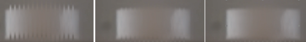
Here’s how we do it. First, we copy several successive frames into an image editing program (I use Xara Designer myself, but I am sure many others, such as Gimp or Inkscape, will work just as well). Then I mask an image of the disc in one of the frames with a comb-like mask, see below (from left to right: mask; masked image; image).

Next, we place a masked image from one frame on top of the unmasked image from the next frame, and begin to move the masked image down in a measurable way (e.g. the displacement can be measured by the number of down-arrow clicks). In the right image below, the slices in the masked and unmasked images coincide almost exactly, so that almost no stripe patterns can be seen near the edges of the slices.
In my enumeration, below are frames 9, 10, and 11.
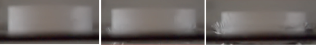
The displacements of the disc as measured in the number of arrow clicks is as follows:
From 3 to 4, from 4 to 5, from 5 to 6: 27 clicks each;
From 6 to 7, from 7 to 8: 28 clicks each;
From 8 to 9: 27 clicks;
From 9 (that is in the left image above) to 10: 19 clicks;
From 10 to 11: 18 clicks
From 11 to 12; 15 clicks.
Based on this data, the impact occurred almost immediately before frame 9. From frame 11 onwards, the added mass has increased so much that the motion is noticeably slowed down. So, in our arbitrary units, u=28 and v=19. From each frame 1-7 we can measure R/h=1.25. All this together gives \rho_{\mathrm{cyl}}\approx 1.12g/cm3. A more accurate result for the density of this cylinder from mass and volume measurements is \rho_{\mathrm{cyl}}\approx 1.14g/cm3.
As promised, we also need to discuss how momentum and energy are carried by sound waves. Suppose we have a sound wave whose displacement of water particles is described by \xi=\xi_0\cos(kx-\omega t). Then the kinetic energy density of the wave is T=\frac 12\rho\dot\xi^2. The total energy density is equal to the maximum value of the kinetic energy (when the potential energy is zero), so E=\frac 12\rho\omega^2\xi_0^2. To find the momentum of the wave, we first express the density variation in the wave: the oscillating part of the density \tilde\rho=\rho\frac{\mathrm d\xi}{\mathrm dx}=\rho k\xi_0\sin(kx-\omega t). The momentum density is given by \tilde\rho\dot\xi; we need its averaged value,
\bar P=\left<\rho k\xi_0\sin(kx-\omega t)\cdot\omega\xi_0\sin(kx-\omega t)\right>=\frac 12\rho\omega k\xi_0^2.In a wave packet, both the momentum and the energy are carried away at the speed of sound c_s, so to obtain the energy and momentum flux we need to multiply the above expressions by c_s. Finally, we can calculate the ratio of the energy and momentum fluxes, Ec_s/\bar Pc_s=\omega/k=c_s. As a side note, the fact that the energy-to-momentum ratio in waves is equal to the phase speed of the waves is used in phonon/plasmon formalisms, making it possible to introduce the number of plasmons, N, and in analogy to quantum mechanics say that the momentum of the waves is N k while the energy is N\omega. Coming back to our case, the total initial energy is on the order of M_{\mathrm{cyl}}v^2, and the momentum is on the order of M_{\mathrm{cyl}}v. Their ratio is on the order of u. Meanwhile, the ratio of the respective wave losses is on the order of c_s\gg v. Therefore, if the energy carried away by the waves is important (and explains the significant reduction in the total kinetic energy of the system during the impact), the momentum losses due to the waves can be ignored with a safe margin, so that our effective conservation of momentum law, derived without considering the propagation of sound waves, can still be used.
We also promised to discuss how quickly the pressure gradient disappears with increasing distance from the disc. As we have seen, the field corresponds to a magnetised ellipsoid. Then the pressure gradient is equal to the magnetic field strength. We are dealing with a dipole field, so the field strength is inversely proportional to the cubed distance.
So what have we learnt? Jumping into water is equivalent to a plastic collision with added mass. So if you jump into water, you will be hit by a rigid lump that moves towards you at your jump speed and has a mass equal to the added mass. If the speed is high, this can be quite dangerous. The value of the added mass depends on how you hit the water. If you have a perfect jump and hit the water with a straight body, and the first part to hit the water is your feet, the added mass can be quite small. Even then, the impact with the added mass becomes dangerous if your jump height exceeds about 30 metres (to be safe, if you are not trained, stay below 3 metres!) That’s why cliff diving competitions include jumps from no higher than about 28 m. However, the mass of the rigid lump with which you collide can be increased many times over if your body orientation and shape at the moment of impact is sub-optimal!